Digital communications systems always represent a collection of design trade-offs. Maximizing one characteristic of a system may impair others, and various communications services may choose to optimize different performance parameters based on the intersection of these design decisions with the physical characteristics of the communications medium.

In this article, I’ll look at the Starlink service¹ and how TCP, the workhorse transport protocol of the Internet, interacts with the characteristics of the Starlink service.

To start, it is useful to recall a small item of Newtonian physics from 1687². On the surface of the Earth, if you fire a projectile horizontally, it will fall back to Earth due to the combination of the effects of the friction from the Earth’s atmosphere and the Earth’s gravitational force. However, assuming that the Earth has no friction-inducing atmosphere, then if you fire this projectile horizontally fast enough, it will not return to the Earth but head into space. If you are high enough to clear various mountains that may be in the way, there is, however, a critical velocity where the projectile will be captured by the Earth’s gravity and neither fall to ground nor head out into space (Figure 1).

This orbital velocity at the surface of the Earth is some 40,320 km/sec. The orbital velocity decreases with altitude, and at an altitude of 35,786 km above the surface of the Earth, the orbital velocity of the projectile relative to a point on the surface of the spinning Earth is 0 km/sec. This is the altitude of a geosynchronous equatorial orbit, where the orbiting object appears to sit at a fixed location in the sky.

Geosynchronous Services

Geosynchronous satellites were the favoured approach for the first wave of satellite-based communications services. Each satellite could “cover” an entire hemisphere. If the satellite was on the equatorial plane, then it was at a fixed location in the sky with respect to the Earth, allowing the use of large antenna. These antennas were able to operate at a low signal to noise ratio, allowing the signal modulation to use an encoding with a high density of discrete phase amplitude points, which lifted the capacity of the service.

All this must be offset against the less favourable aspects of a geosynchronous service. Consideration of crosstalk interference between adjacent satellites in geosynchronous orbits using the same radio frequencies resulted in international agreements that require a 2° spacing for geosynchronous satellites that use the same frequency, so this orbital slot is a limited resource that is limited to just 180 spacecraft if they all use K band (18 - 27Ghz) radio systems. At any point on the Earth, there is an upper bound to the signal capacity that can be received (and sent) using geosynchronous services.

Depending on whether the observer is on the equator directly beneath the satellite or further away from this point, a geosynchronous orbit satellite is between 35,760 and 42,664 km away, so a signal round trip time to the geosynchronous satellite and back will be between 238ms and 284ms in terms of signal propagation time. In IP terms, that’s a round trip time of between 477 and 569ms, and signal encoding and decoding times need to be added to this. In addition, there is a delay in the signal being passed between the terrestrial endpoints and the satellite earth stations. In practice, a round trip time of around two-thirds of a second (660ms) for Internet paths that include a geosynchronous satellite service is a common experience.

This extended latency means that the endpoints need to use large buffers to hold a copy of all the unacknowledged data, as is required by the TCP protocol. TCP is a feedback-governed protocol that uses ACK pacing. The longer the round time, the greater the lag in feedback, and the slower the response from endpoints to congestion or to available capacity. The congestion considerations lead to the common use of large buffers in the systems driving the satellite circuits, which can further exacerbate congestion-induced instability. In geosynchronous service contexts, individual TCP sessions are more prone to instability and experience longer recovery times following low events than their terrestrial counterparts when such counterparts exist³.

Low Earth Orbit Systems

A potential response to the drawbacks of geosynchronous satellites is to bring the satellite closer to Earth. This approach has several benefits. The Earth’s spinning iron core generates a magnetic field, which traps energetically charged solar particles and redirects them through what is called the “Van Allen Belt,” thus deflecting solar radiation. Not only does this allow the Earth to retain its atmosphere, but it also protects the electronics of orbiting satellites that use an orbital altitude below 2,000 km or so from the worst effects of solar radiation (such as the recent solar storms). It’s also far cheaper to launch satellites into a low earth orbit, and these days SpaceX is able to do so using re-usable rocket boosters.

The reduced distance between the Earth and the orbiting satellite reduces the latency in sending a signal to the satellite and back, which can improve the efficiency of the end-to-end packet transport protocols that include such satellite circuits.

This group of orbital altitudes, from some 160km to 2,000km, are collectively termed Low Earth Orbit (or LEOs)⁴. The objective here is to keep the satellite’s orbit high enough to prevent it from slowing down by grazing the upper parts of the Earth’s ionosphere, but not so high that it loses the radiation protection afforded by the Inner Van Allen belt⁵. At a height of 550km, the minimum signal propagation delay to reach the satellite and back from the surface of the Earth is just 3.7ms.

But all of this comes with some different issues. At a height of 550km an orbiting satellite can only be seen by a small part of the Earth. If the minimum effective elevation to establish communication is 25 degrees of elevation above the horizon, then the satellite’s footprint is a circle with a radius of 940km, or a circle of area 2M km2. (Lower angles of elevation are possible, but the longer the path segment through the Earth’s atmosphere decreases the signal-to-noise ratio, compromising the available signal capacity as well as increasing the total path delay.) To provide continuous service to any point on the Earth’s surface (510.1M km2) the minimum number of orbiting satellites is 500. This use of a constellation of satellites implies that a LEO satellite-based service is not a simple case of sending a signal to a fixed point in the sky and having that single satellite mirror that signal down to some other earth location. A continuous LEO satellite service needs to hop across a continual sequence of satellites as they pass overhead and switch the virtual circuit path across to successive satellites as they come into view of both the end user and the user’s designated earth station.

At an altitude of 550 km, an orbiting satellite is moving with a relative speed of 27,000 km/hour relative to a point on the Earth’s surface and passes across the sky from horizon to horizon in under 5 minutes. This has some implications for the design of the radio component of the service. If the satellite constellation is large enough, then the satellites are close enough to each other that there is no need to use larger dish antennae that require some mechanized steering arrangement that tracks individual satellites in their path across the sky, but this itself is not without its downside. An individual signal carrier might be initially acquired as a weak signal (in relative terms), increases in strength as the satellite’s radio transponder and the Earth antenna move into alignment, and weakens again as the satellite moves on. Starlink’s antennae use a phased array arrangement using a grid of smaller antennae on a planar surface. This allows the antenna to be electronically steered by altering the phase difference between each of the antennae in the grid. Even so, this is a relatively coarse arrangement, so the signal quality is not consistent. This implies a constantly varying Signal to Noise Ratio (SNR) as the phased array antenna tracks each satellite during its overhead path.

It appears that Starlink services use dynamic channel rate control as a response to this constantly varying SNR. The transmitter constantly adjusts the modulation and coding scheme to match the current SNR, as described in the IEEE 802.11ac standard. The modulation of this signal uses adaptive phase amplitude modulation, and as the SNR improves the modulator can use a larger number of discrete code points in this phase amplitude space, thus increasing the effective capacity of the service while using a constant frequency carrier signal. What this implies is that the satellite service is attempting to operate at peak carriage efficiency, and to achieve this, the transmitter constantly adapts its signal modulation to take advantage of the instantaneous SNR from the satellite system. To the upper layer protocol drivers, the transmission service appears to have a constantly varying channel capacity and latency.

The Starlink satellite’s Ku-band downlink has a total of 8 channels using frequency division multiplexing. Each channel has an analogue bandwidth of 240Mhz. Each channel is broken into frames, which is subdivided using time division multiplexing into 302 intervals, each of 4.4µs, which together with a frame guard interval makes each frame 1,333µs, or 750 frames per second. Each frame contains a header that contains satellite, channel and modulation information⁶. The implication is that there is a contention delay of up to 1.3ms, assuming that each active user is assigned at least one interval per frame.

This leaves us with four major contributory factors for variability of the capacity of the Starlink service, namely:

• the variance in signal modulation capability, which is a direct outcome of the varying SNR of the signal,
• the variance in the satellite path latency due to the relative motion of the satellite and the earth antennae,
• the need to perform satellite switching on a regular basis, and
• the variability induced by sharing the common satellite transmission medium with other users, which results in slot contention.

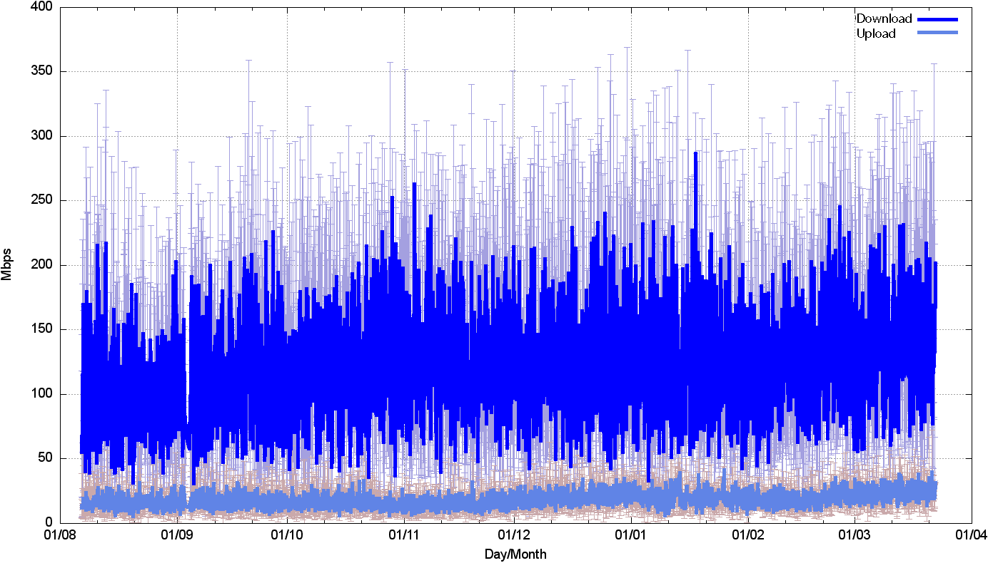
One way to see how these variability factors impact the service characteristics is to use a capacity measurement tool to measure the service capacity on a regular basis. The results of such a capacity measurement test in a Starlink service are shown in Figure 2. Here, the test is a SpeedTest measurement test⁷, performed on a 4-hourly basis for the period August 2023 through March 2024. The service appears to have a median value of around 120Mbps of download capacity, with individual measurements reading as high as 370Mbps and as low as 10Mbps, and 15Mbps of upload capacity, with variance of between 5Mbps to 50Mbps.

In Internet terms, ping⁸ is a very old tool, but at the same time, it’s still a very useful tool, which probably explains its longevity. Figure 3 is a plot of a continuous (flood) ping across a Starlink connection from the customer side terminal to the first IP endpoint behind the Starlink earth station for a 380-second interval. (A “flooding” ping sends a new ping packet each time a packet is received from the remote end).

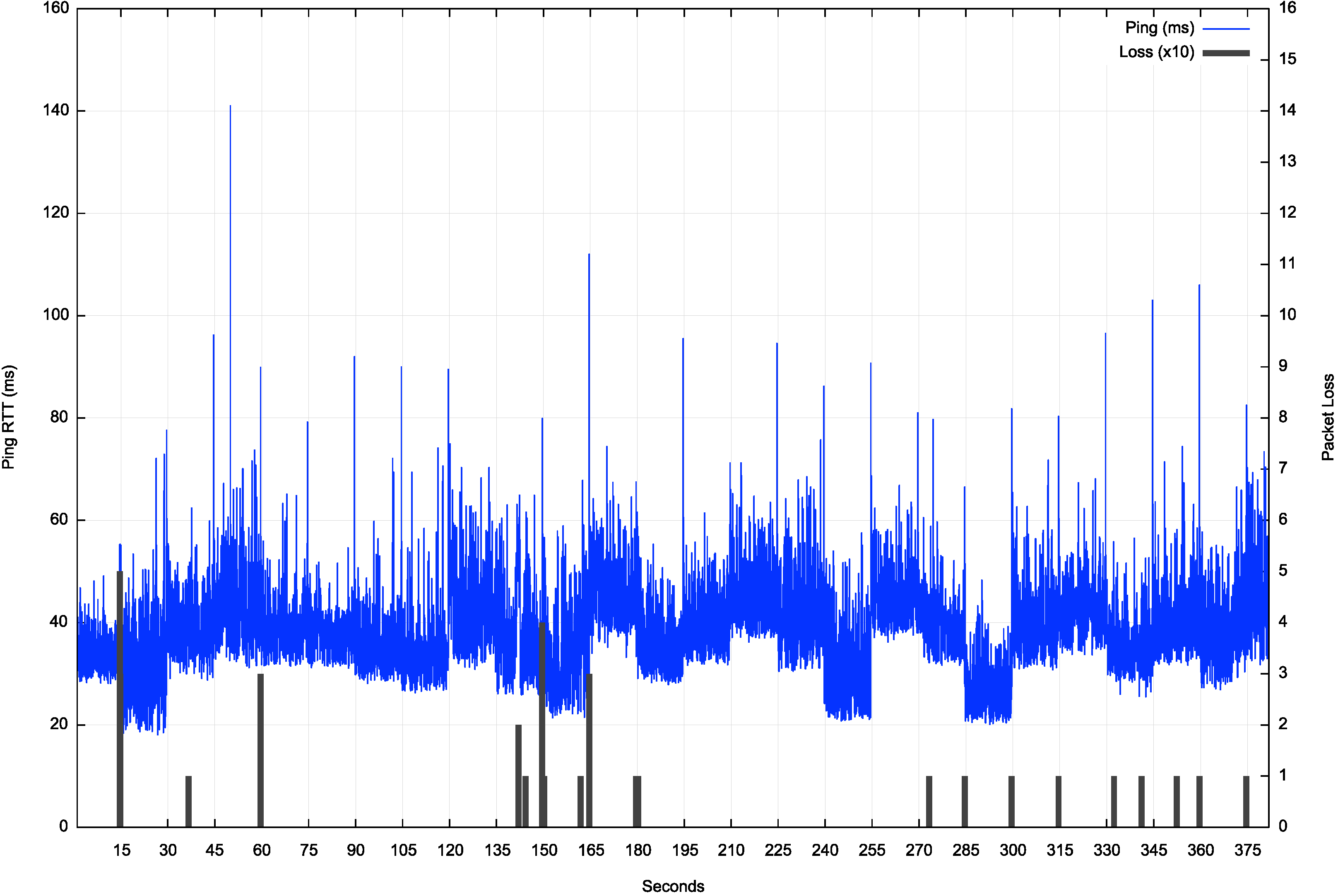
The first major characteristic that is visible in this ping data is that the minimum latency changes regularly every 15 seconds. It appears that this change correlates to the Starlink user’s terminal being assigned to a different satellite. That implies that the user equipment “tracks” each satellite for a 15 second interval, which corresponds to a tracking angle of 11 degrees of arc.

The second characteristic is that loss events are seen to occur at times of switchover between satellites, as well as occurring less frequently as a result of either obstruction, signal quality or congestion.

The third is that there is a major increase in latency at the point when the user is assigned to a different spacecraft. The worst case in this data set is a shift from 30ms to 80ms.

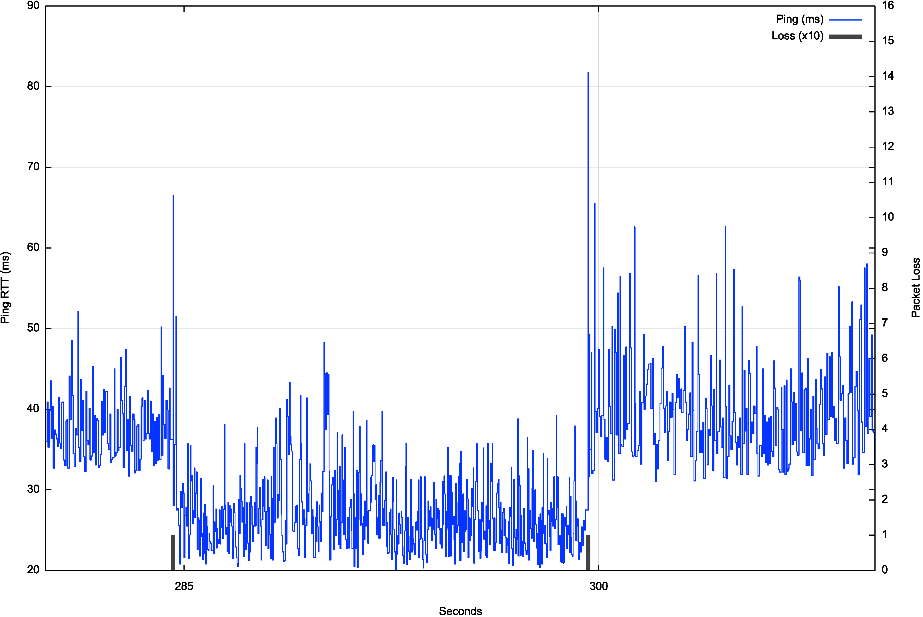
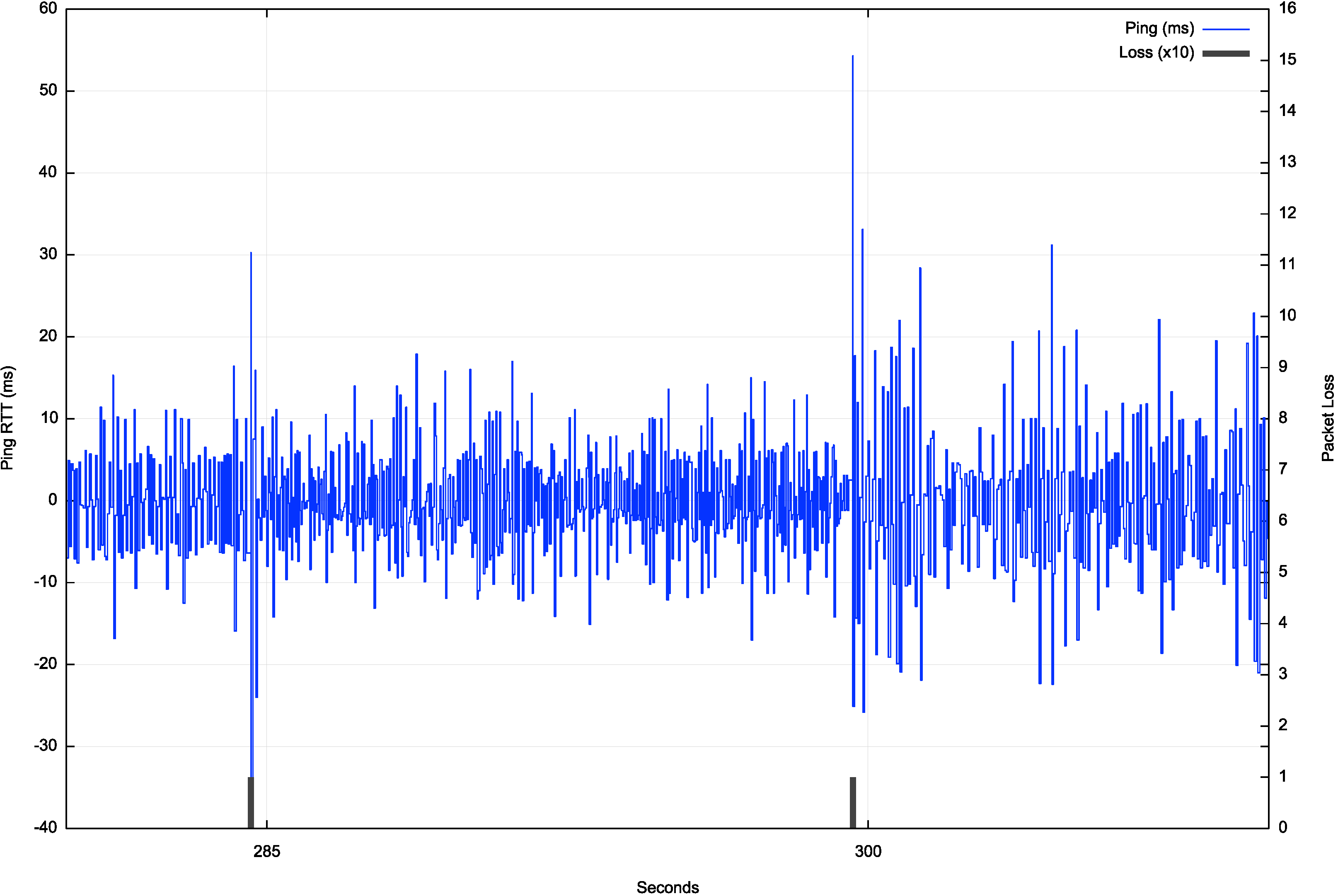
Finally, within each 15s satellite tracking interval, the latency variation is relatively high. The average variation of jitter between successive RTT intervals is 6.7ms. The latency spikes at handover impose an additional 30ms to 50ms indicating the presence of deep buffers in the system to accommodate the transient issues associated with satellite handover. To illustrate this link behavior, the ping data set has been filtered to remove the effects of the satellite assignment at second 283 and second 298. (Figure 5).

The overall packet loss rate, when measuring using 1-second paced pings over an extended period is a little over 1% as a long-term average loss rate.

TCP Protocol Performance

TCP⁹ is an instance of a sliding window positive acknowledgment protocol. The sender maintains a local copy of all data that has been passed into the local system’s IP layer and will only discard that local copy of sent data when it has received a positive acknowledgement from the receiver.

Variants to TCP are based on the variations in the sender’s control of the rate of passing data into the network and variations in the response to data loss. The classic version of TCP uses a linear inflation of the sending window size while there is no loss, and it halves this window in response to packet loss. This is the RENO TCP control algorithm. Its use in today’s Internet has been largely supplanted by the CUBIC TCP control algorithm¹⁰, which uses a varying window inflation rate that attempts to stabilize the sending rate at a level just below the build-up of network queues (which ultimately leads to packet loss).

In general terms, there is a small set of common assumptions about the characteristics of the network path for such TCP control algorithms:

• There is a stable maximal capacity of the path, where the term stability describes a situation where the available path capacity is relatively constant across a number of RTT intervals.
• The amount of jitter (variation in end-to-end delay) is low in proportion to the RTT.
• >The average packet loss rate is low. In the case of congestion-based loss TCP control algorithms packet loss is generally interpreted by the algorithm as a sign that the network’s buffers have filled, and loss is an indication of buffer overflow.

Obviously, as we’ve noted, the first two conditions do not necessarily hold for end-to-end paths that include a Starlink component. The loss profile is also different. There is the potential for congestion-induced packet loss, as is the case in any non-synchronous packet switched medium, but there is an additional loss component that can occur during satellite handover, and a further loss component that can be caused by other impairments imposed upon the radio signal.

TCP typically tends to react to such environments by using conservative choices.

The RTT estimate is a smoothed average value of RTT measurements, to which the mean deviation of individual measurements from this average is added. For Starlink, with its relatively high level of individual variance in RTT measurements this means that the TCP sender may operate with a RTT estimate that is higher than the minimum RTT, which may result in a sending rate that is lower than the available end-to-end capacity of the system.

The occurrence of non-congestion-based packet loss can also detract from TCP performance. Conventionally, the loss will cause the sender to quickly reduce it’s sending window on the basis that if this loss is caused by network buffer overflow, then the sender needs to allow these buffers to drain, and then it will resume sending at a lower rate, which should restore coherency of the feedback control loop.

How does this work in practice?

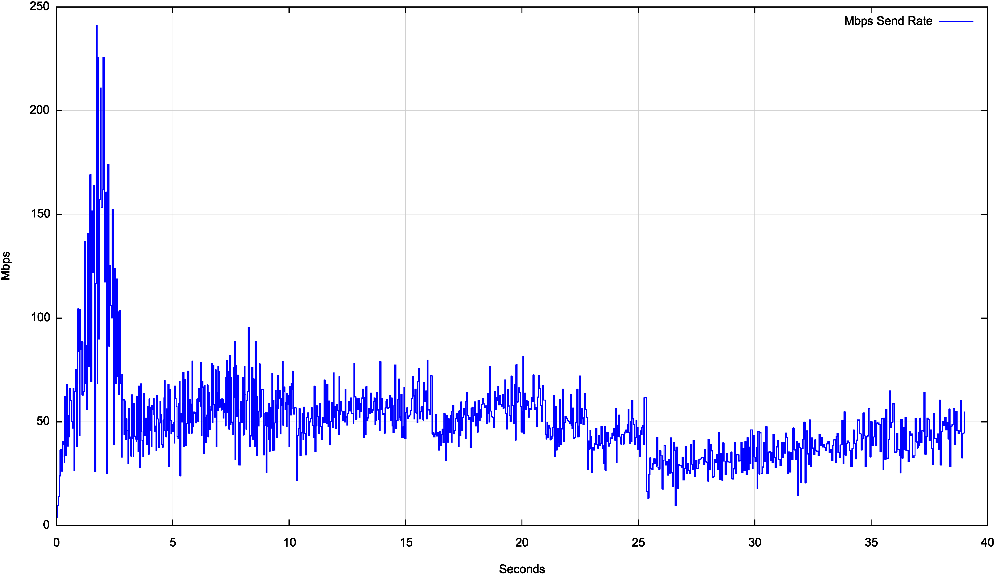
Figure 6 shows a detailed view of a TCP cubic session over a Starlink circuit. The initial 2 seconds shows the slow start TCP sending rate inflation behaviour, where the sending window doubles in size for each RTT interval, reaching a peak of 240Mbps in 2 seconds. The sender then switches to a mode of rapid reduction of the sending window in the next second, dropping its sending rate to 50Mbps within one second. At this point, the CUBIC congestion avoidance phase appears to kick in, and the sending rate increases to 70Mbps over the ensuing 5 seconds. There is a single loss event which cases the sending rate to drop in second 8 back to 40Mbps. The remainder of the trace shows this same behavior of slow sending rate inflation and intermittent rate reductions, which is typical of CUBIC.

This CUBIC session managed an average transfer rate of some 45Mbps, which is well below the peak notional circuit capacity of some 250Mps, as indicated by SpeedTest.

Starlink is a shared medium, and the performance of the system in local times of light use (off-peak) is significantly different from the performance in peak times. Figure 7 shows CUBIC performance profile during an off-peak time.

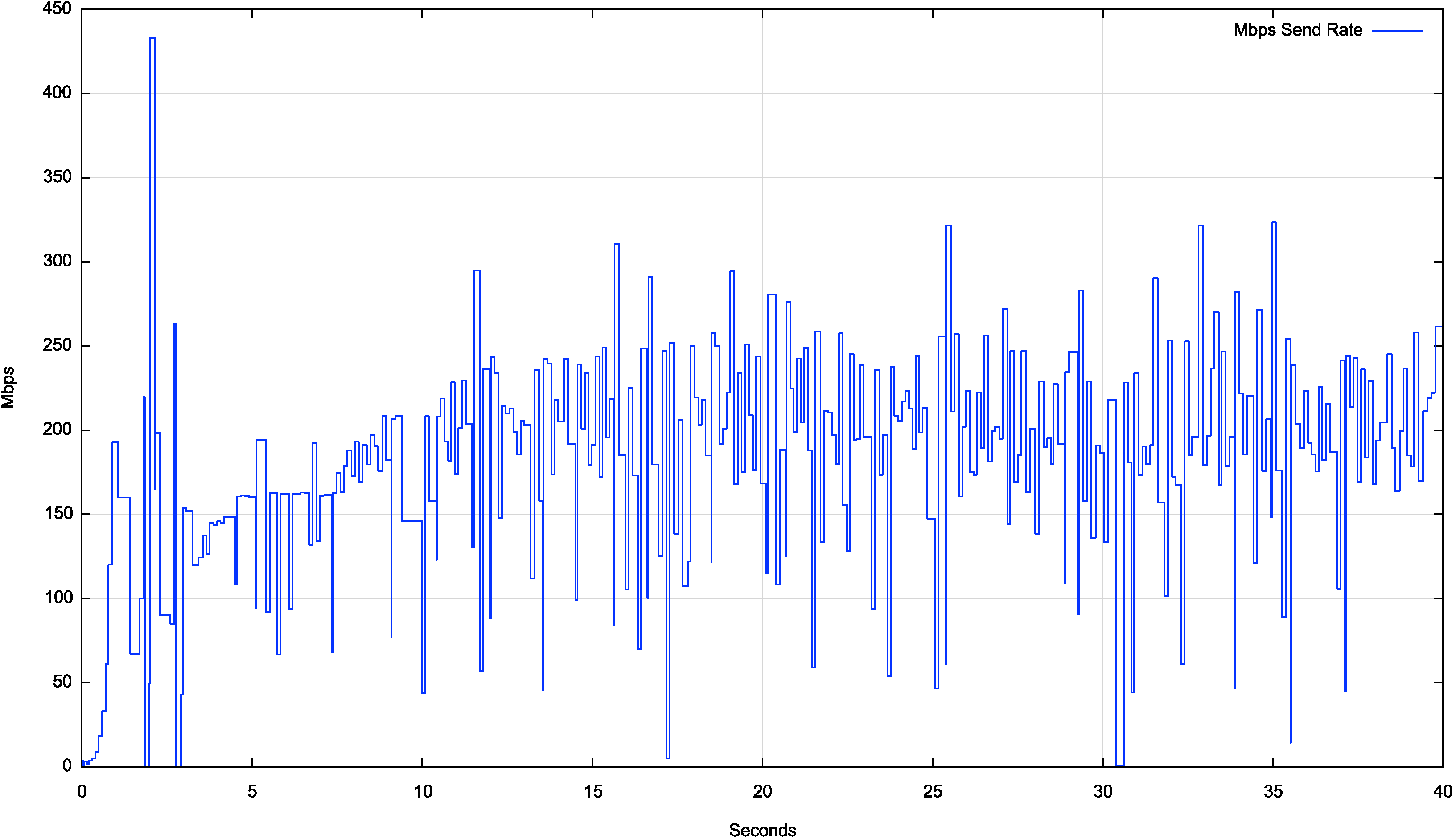
The difference between the achievable throughput between peak and off-peak is quite significant, with the off-peak performance reaching a throughput level some 3—4 times greater than the peak load performance. The slow-start phase increases the throughput to some 200Mbps within the first second. The flow then oscillated for a second, then started a more stable congestion avoidance behavior by second 4. The cubic window inflation behavior is visible up to second 12, and then the flow oscillates around some 200Mbps of throughput for the remainder of the session.

Is the difference between these two profiles in Figures 6 and 7 a result of active flow management by Starlink equipment or the result of the way in which CUBIC reaches a flow equilibrium with other concurrent flows?

We can attempt to answer this question by using a different TCP control protocol that has a completely different response to contention from other concurrent flows.

The Bottleneck Bandwidth and Round-trip propagation time (BBR) protocol¹¹ is a TCP congestion control algorithm developed at Google a decade or so ago. BBR attempts to position the TCP flow at the onset of network queue formation rather than oscillating between full and empty queue states (as is the case in most loss-based TCP congestion control algorithms).

Briefly, BBR makes an initial estimate of the delay-bandwidth product of the network path, and then drives the sender to send at this rate for 6 successive RTT intervals. It performs repair for dropped packets without adjusting its sending rate. The 7th RTT interval sees the sending rate increase by 25%, and the end-to-end delay is carefully measured. The final RTT interval in the cycle sees the sending rate drop by 25% from the original rate, intended to drain any network queues that may have formed in the previous RTT interval. If the end-to-end delay increases in the sending rate inflated interval, the original sending rate is maintained. If the increased sending window did not impact the end-to-end delay, then this indicates that the network path has further capacity and the delay-bandwidth estimate is increased for the next 8-RTT cycle. (There have been a couple of subsequent revisions to the BBR protocol, but in this case, I’m using the original (v1) version of BBR.)

The results of a Starlink performance test using BBR is shown in Figure 8.

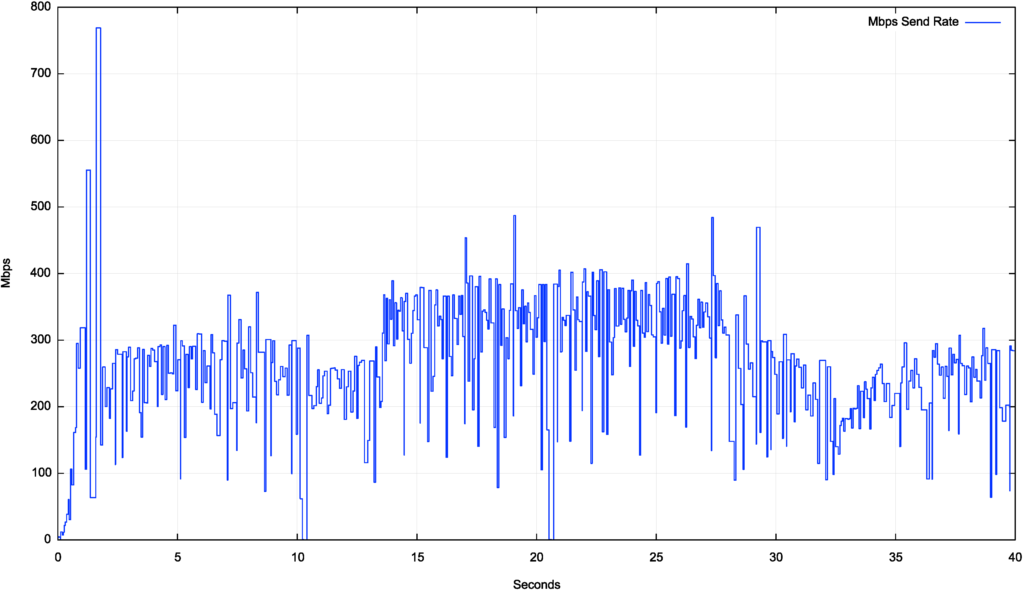
In this case, BBR has made an initial estimate of some 250Mbps for the path bandwidth. This estimate appears to have been revised at second 14 to some 350Mbps and then dropped to some 200Mbps some 15 seconds later for the final 10 seconds of this test. It is likely that these changes are the result of BBR responding to satellite handover in Starlink, and BBR interpreted the variance in latency as a sign of queue formation, or the absence of queue formation, which was used to alter BBR’s bandwidth delay estimate for the link.

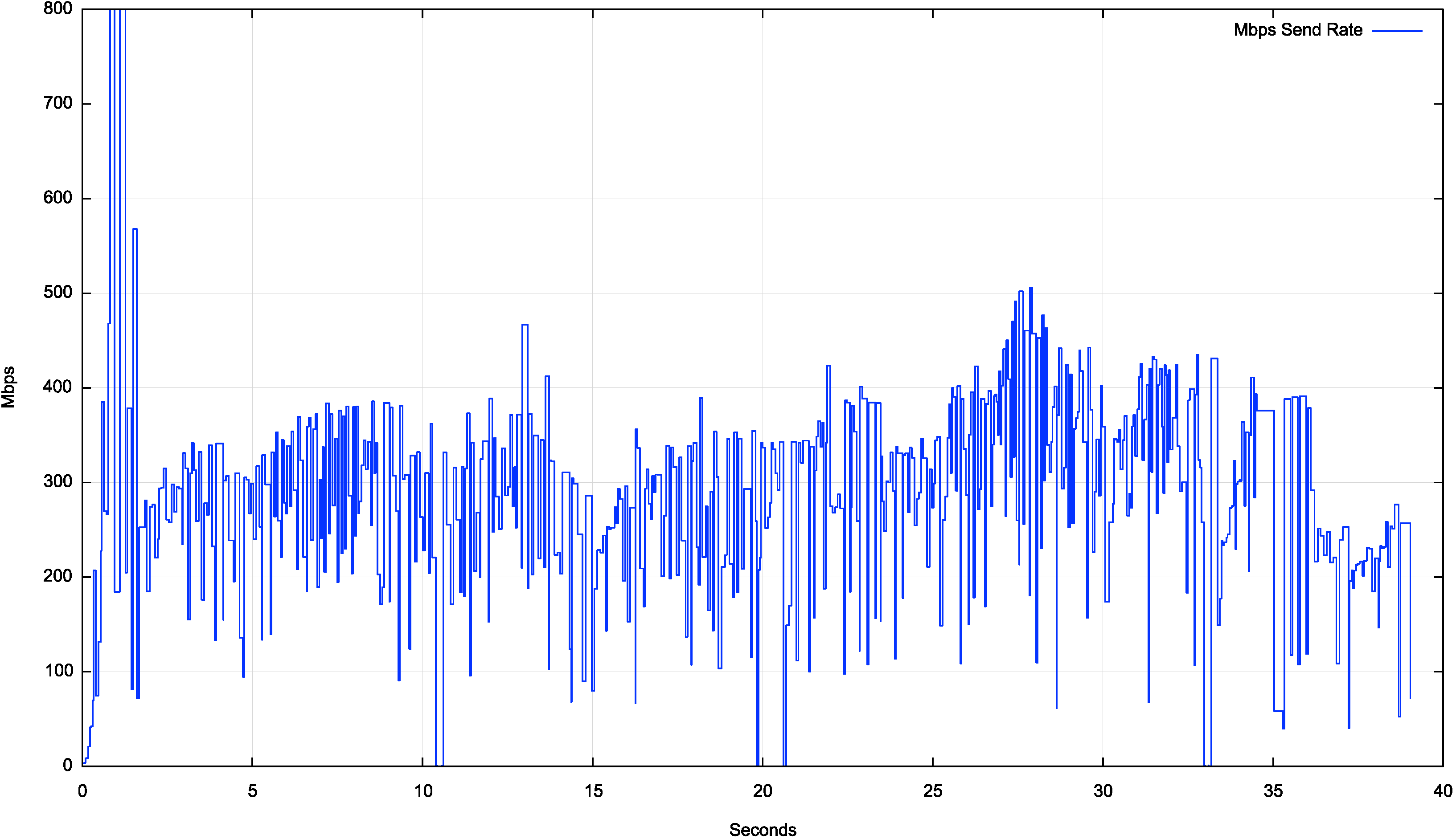
The same BBR test was performed during an off-peak time, which resulted in a very similar outcome (Figure 9).

If BBR is sensitive to changes in latency, and latency is so variable in Starlink, then why does BBR perform so well as compared to CUBIC?

I suspect that here, BBR is not taking a single latency measurement but measuring the round-trip time for all packets that are sent in this 7th RTT interval once the sender has increased its sending rate to the burst rate and uses the minimum RTT value as the ‘loaded’ RTT value to determine whether to perform a send rate adjustment. As long as the minimum RTT levels are consistent, and, as shown in Figure 3, these minimum values appear to be consistent across each 15-second scheduling interval, then BBR will assume that its sending rate is not causing network queue formation and will maintain its sending rate.

Protocol Tuning for Starlink

Starlink provides a somewhat unique data link service. It has a very high jitter rate, a packet drop rate of around 1%-2% that is unrelated to network congestion, and a latency profile that jumps on a regular basis every 15 seconds. From the perspective of the TCP protocol, Starlink represents an unusually hostile link environment, and older variants of TCP, such as Reno TCP, that react quickly to packet loss and recover slowly, can perform very poorly when used across Starlink connections.

Could you tune a variant of TCP to optimize its performance over a path that includes a Starlink component?

A promising approach would appear to start with a variant of BBR. The reason for choosing BBR is its ability to maintain its sending rate in the face of individual packet loss events. If one were to optimize BBR for Starlink, then it can be noted that Starlink performs a satellite handover at regular 15-second intervals, and if the regular sending rate inflation in BBR occurs at the same time as the scheduled satellite handover, the BBR sender could defer its rate inflation, maintaining its current sending rate across the scheduled handover time.

The issue with BBR is that, for version 1 of this protocol, it is quite aggressive in claiming network resources, which can starve other non BBR TCP concurrent sessions of capacity. One possible response is to use the same 15-second satellite handover timer with version 3 of the BBR protocol, which is intended to be less aggressive when working with concurrent data flows.

In theory, it would be possible to adjust CUBIC in a similar manner, performing a lost packet repair using Selective Acknowledgement (SACK)¹¹ if the packet loss occurred at the time of a scheduled satellite handover. While CUBIC is a fairer protocol with respect to sharing the path capacity with other concurrent TCP sessions, it tends to react conservatively when faced with high-jitter paths (as is the case when the end-to-end path includes a Starlink component). Even with some sensitivity to scheduled satellite handovers, CUBIC is still prone to reduced efficiency in the use of network resources.

A somewhat different approach could utilize Explicit Congestion Notification (ECN)¹². The advantage of such an approach is that it allows the TCP session to differentiate the case where a high sending rate it causes the formation of network queues (congestion), while a transient event, such as satellite handover, causes packet loss without network queue formation. ECN can permit a flow control behavior that is very much like BBR.

Conclusions

While earlier TCP control protocols, such as Reno, have been observed to perform poorly on Starlink connections, more recent TCP counterparts, such as CUBIC, perform more efficiently. The major TCP feature that makes these protocols viable in Starlink contexts is the use of Selective Acknowledgement¹¹, which allows the TCP control algorithm to distinguish between isolated packet loss and loss-inducing levels of network congestion.

TCP control protocols that attempt to detect the onset of network queue formation can do so using end-to-end techniques by detecting changes in end-to-end latency during intermittent periods of burst, such as BBR. These protocols need to operate with a careful implementation of their sensitivity to latency, as the highly unstable short-term latency seen on Starlink connections, coupled with the 15-second coarse level latency shifts have the potential to confuse the queue onset detection algorithm.

It would be interesting to observe the behavior of an ECN-aware TCP protocol behavior if ECN were to enabled on Starlink routing devices. ECN has the potential to provide a clear signal to the endpoints about the onset of network-level queue formation, as distinct from latency variation.